原点に対して空間反転の操作を行えば、 にあった座標は
  へ移される(原点について点対称)。 これは量子力学などの物理ではパリティ変換(反転)として知られ、空間座標の符号を変換する。
たとえば、原子に一様な電場をかけた場合にエネルギー準位が分裂する(シュタルク効果)を考える際にもこの対称性は使われる。
空間反転
直交座標と極座標の場合について見ていく。
直交座標の成分
空間反転により  と変換される。
 を直交座標系で書くと、空間反転の操作
  により
により

に移される。この操作 を3 3の行列で表現すれば

である。 となる。通常の軸周りの回転を表す行列
  ,
,  ,
,  を組み合わせて を作ることはできない。なぜなら、

は  であるためである。たとえば、直交行列に関して行列式の性質から
![\begin{eqnarray*} {\rm det}[R_xR_yR_z]={\rm det}R_x\cdot {\rm det}R_y \cdot {\rm det}R_z=1 \end{eqnarray*}](https://batapara.com/wp-content/ql-cache/quicklatex.com-3c2734538082ecc01887552922912082_l3.png "Rendered by QuickLaTeX.com")
となる。
極座標の成分
を極座標表示で表すと

この式から  がどのように変換されるか見ていく。そのあとで、図を書いて の関係を見ていく。
空間反転に対してベクトルの大きさ変化しない ( ) ので
) ので  である。次に
  について見てみると、
 成分について
  でないといけない。
 は変化しないので、

である。したがって、 と変換される。最後に
  について見ていく。
 成分が
成分が  となるためには、

でなくてはならない。したがって、 となる。
となる。
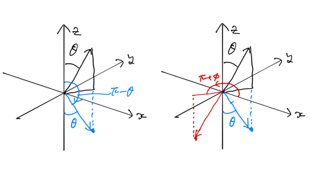
これらの結果をまとめると極座標について

となる。このことを下の図に表した。まず、 平面に対して反転操作を行い(左図)、 軸に対して反時計回りに
  回転すれば(右図)、空間反転に対応することが確認できる。この操作はその性質上、 軸回転から始めて、 平面の反転をとっても同様の結果になる。
パリティ
以下ではパリティ反転(空間座標を反転させる操作)を表す演算子を  とする。つまり、ある関数
  に対して
に対して

となる演算子 について考える。
* 式(1)は固有値方程式ではない。固有値方程式は  の形で、両辺に現れる関数は同じ形でないといけない。以下では、 の固有値・固有関数を考える。
固有値・固有関数
の固有値  を考える。固有関数を
  とすると
とすると

である。両辺にさらに を左から作用させて、

式(1)より  を用いると、左辺は

となる。したがって、 から
から  となる。固有値 に対して固有関数
  と書くと、
と書くと、

一方、式(1)より  の関係を用いて左辺を書き直すと

これより、 は偶関数(パリティが偶)、
 は奇関数(パリティが奇)となる。任意の関数はこの2つの
  で展開することができ、完全系をなす。
水素原子のハミルトニアンとの交換関係
水素原子のシュレディンガー方程式について、電子の受けるポテンシャルは原子からのクーロンポテンシャルのみで球対称になっている。したがって、ポテンシャルは  の関数であり、角度によらないポテンシャルになる。
直交座標系で書いたハミルトニアンは、

となる。ここで、空間反転  について球対称ポテンシャルは以下のように形を変えない。

また、 などの部分について、
![\begin{eqnarray*} \frac{\partial^2}{\partial x^2}\to\frac{\partial}{\partial (-x)}\left[\frac{\partial}{\partial (-x)}\right]=+\frac{\partial^2}{\partial x^2} \end{eqnarray*}](https://batapara.com/wp-content/ql-cache/quicklatex.com-97456403cc0eb0837757e51deac0be4b_l3.png "Rendered by QuickLaTeX.com")
より、空間反転に対して不変である。したがって、上の  は空間反転に対して不変である。極座標表示したハミルトニアンでも同様の結果になる。ハミルトニアンが空間反転に対して不変であるので、交換関係は
![\begin{eqnarray*} [{\hat{\mathcal P}},\hat{\mathcal H}]=0 \end{eqnarray*}](https://batapara.com/wp-content/ql-cache/quicklatex.com-f29b799c789ef1b1e67778303beda108_l3.png "Rendered by QuickLaTeX.com")
となる。
![[{\hat{\mathcal P}},\hat{\mathcal H}]=0](https://batapara.com/wp-content/ql-cache/quicklatex.com-96eda97e6d8febdcc36f57f42e943d87_l3.png "Rendered by QuickLaTeX.com") を示す。
を示す。
まず
の固有関数を  とする。このとき、 が空間反転に対して対称なので

である。また、
 であるため、

となり、
となる。
 が交換するため と は同時固有状態をもつ。 の固有状態は、水素原子における電子の波動関数 であり、動径波動関数
  と球面調和関数
  の積で表されていた。したがって、 の固有関数である
  は の固有関数でもある(同時固有状態)。よって

となる。波動関数のパリティ( が偶関数か奇関数か)によって固有値 が異なる。あとで示されるように  であり、パリティは量子数
  のみ依存することがわかる。

 に対応する
に対応する  軌道、
軌道、 軌道、
軌道、 軌道はそれぞれ同じ で指定される球面調和関数 の線形結合で表される。したがって、上のパリティはそのまま、
 軌道のパリティに対応する。たとえば、
 の 軌道, 軌道に対しては偶パリティで、
 の 軌道,
の 軌道,  軌道は奇パリティである。
球面調和関数のパリティ
最後に、 となることを示す。 の空間反転において、 より動径関数 は偶関数となる。これより

について  に対する偶奇を調べる。まず、

となる。次にルジャンドル陪多項式  について考える。ルジャンドル多項式
  はロドリゲスの公式より

と書ける。 を用いて  は
は

となる。 に対して、
に対して、

となる。この結果と(2)より は  に対して
に対して

となる。これより
